GRASS GIS

The first thing to do when starting to work in GRASS is to create a Location. GRASS Locations are single projection areas with a defined resolution and extent. The initial location can be easily created from an existing data set.

GRASS DataBase Structure

The GRASS database structure contains three levels:

1. DataBase is a directory on local or network disc which contains all data accessed by GRASS. It’s usually directory called “grassdata” located in user’s home directory.
2. Location is a subdirectory in DataBase which plays a role of project area. All geospatial data stored within one location must have the same spatial coordinate system. Location also defines default computational region.
3. Mapset is a subdirectory in a location. It helps to organize maps into logical groups or to separate parallel work of more users on the same project (within one location).

When starting GRASS you must to define all these three items, see figure bellow.

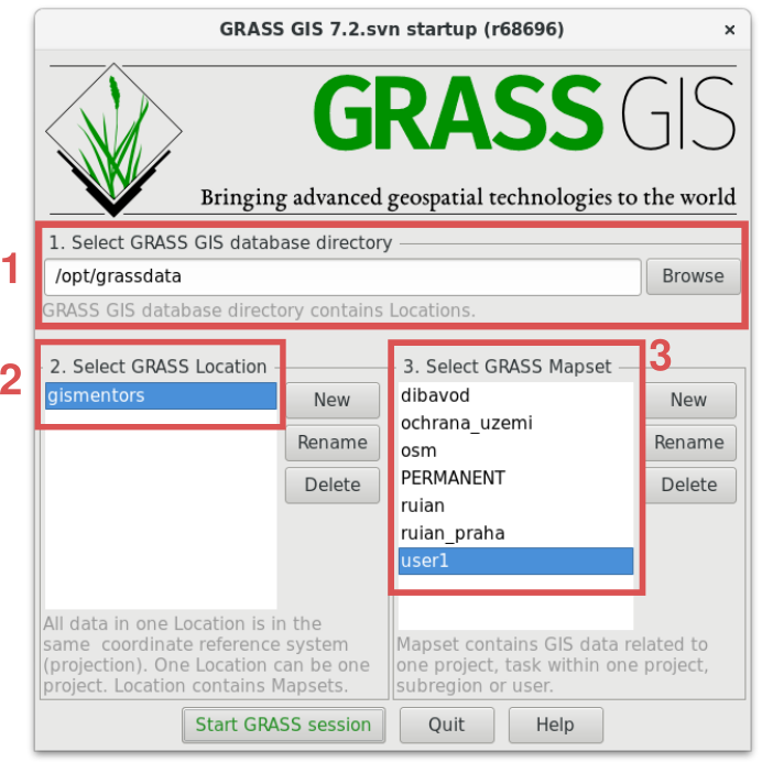
Fig. 11 GRASS startup screen to choose database, location, and mapset.

The user have write permission only to the current mapset, maps from other mapsets within one location can be read without restrictions (if not defined on OS level), see figure bellow. The list of visible mapsets can be modified in menu Settings ‣ GRASS working environment ‣ Mapset access.

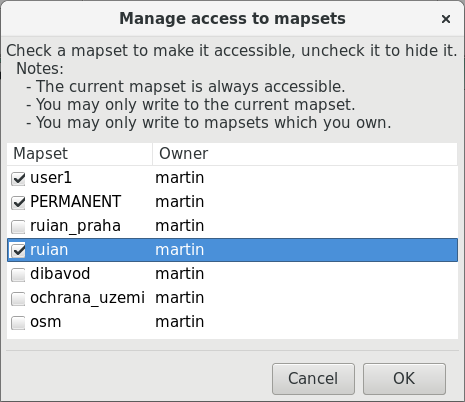
Fig. 12 Dialog for modifying mapset search path.

Accessing maps from other locations requires to reproject selected map by r.proj (raster maps) or v.proj (vector maps). GRASS doesn’t support so-called reprojection-on-the-fly.

GRASS can be started by specifying full path to the mapset from command line

grass72 /opt/grassdata/gismentors/user1

Creating new location

You can create new location when starting GRASS, or from running session in the menu Settings ‣ GRASS working environment ‣ Create new location.

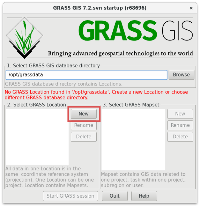
Fig. 13 Create new location from startup screen.

In the location wizard you define name for new location.

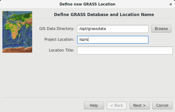
Fig. 14 Name for a new location.

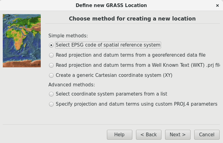
Fig. 15 Methods for creating a new location.

We will choose mostly used method based on well-known EPSG code, in our case UTM zone 33N - EPSG:32633.

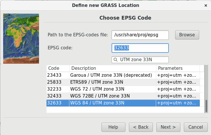
Fig. 16 Creation of new location with EPSG code 32633.

When the new location is created you can choose it from the GRASS startup screen.

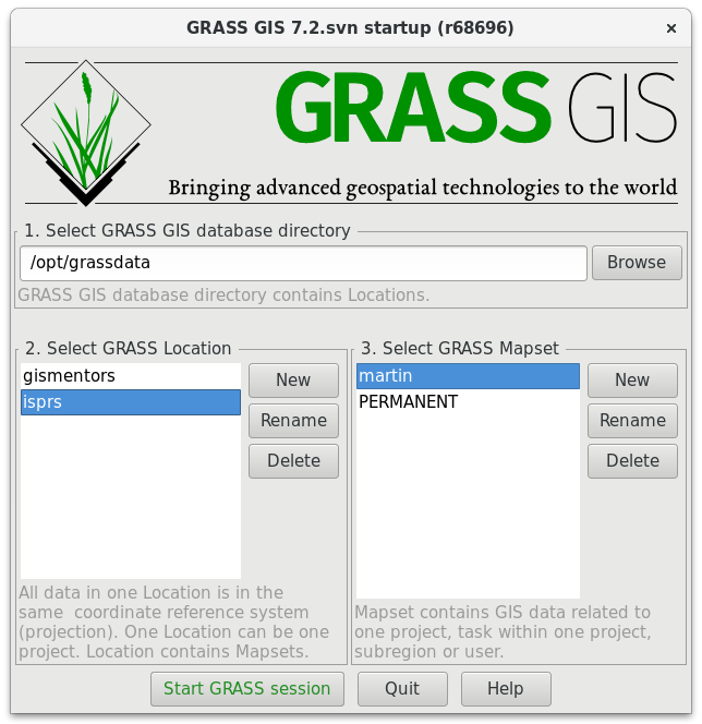
Fig. 17 New location accessible via GRASS startup screen.

New GRASS location can be also created from command line

grass72 -c EPSG:32633 ~/grassdata/isprs/PERMANENT

Import vector data

Dialog for importing vector data is accessible from menu File ‣ Import vector data ‣ Common import formats, from the main toolbar, or from command line using v.import module.

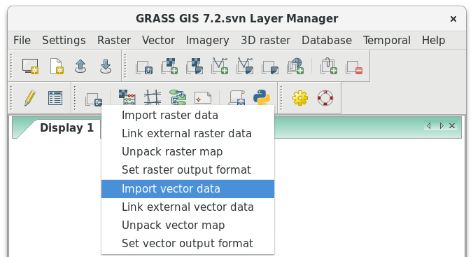
Fig. 18 Import vector data from the main toolbar.

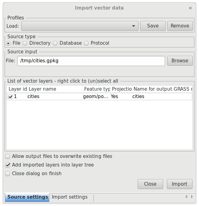
Fig. 19 Example of importing vector layer from OGC GeoPackage file.

Note for advanced users

Import process can take a while. GRASS is a topological GIS. It means that importing vector data doesn’t mean only converting data from one data format to another, but mainly converting from simple feature model to GRASS topological model, see figure bellow.

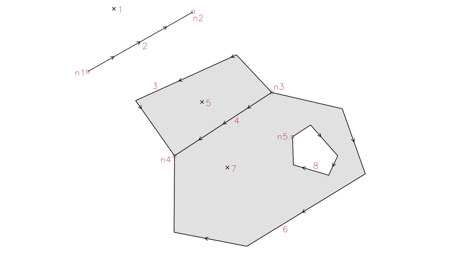
Fig. 20 GRASS topological model.

During this process also topological errors are checked and repaired. Some topological errors is not possible to repair automatically without user specification, in this case the user can fix remaining error using v.clean.

Import raster data

Raster data is possible to import from the menu File ‣ Import raster data ‣ Common import formats, from the main toolbar, or from command line using r.import module.

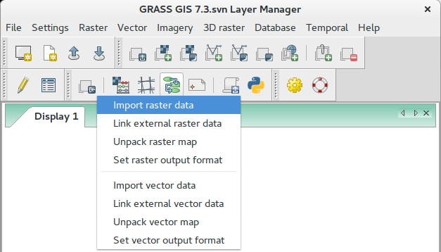
Fig. 21 Import raster data from the main toolbar.

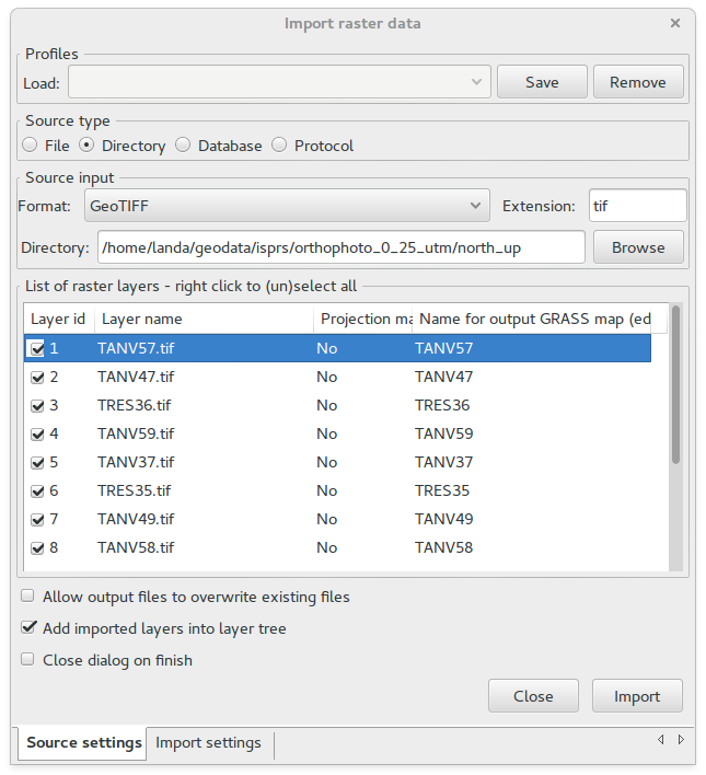
Fig. 22 Example of importing raster files in GeoTIFF format from directory. Since raster files lack spatial reference information (project doesn’t match) we will force overriding project check (Import settings ‣ Optional ‣ Override projection check).

Note for advanced users

To avoid data duplication GRASS also allows linking raster data using r.external (Link external raster data).

Note

GRASS imports raster bands as separate raster maps. Raster maps are represented by regular grid. Three different types are supported:

• CELL (integer)
• FCELL (float)
• DCELL (double)

Working with GUI

GRASS GUI consists of two main windows:

• Layer Manager (1.)
• Map Display (user can run multiple Map Display windows) (2.)

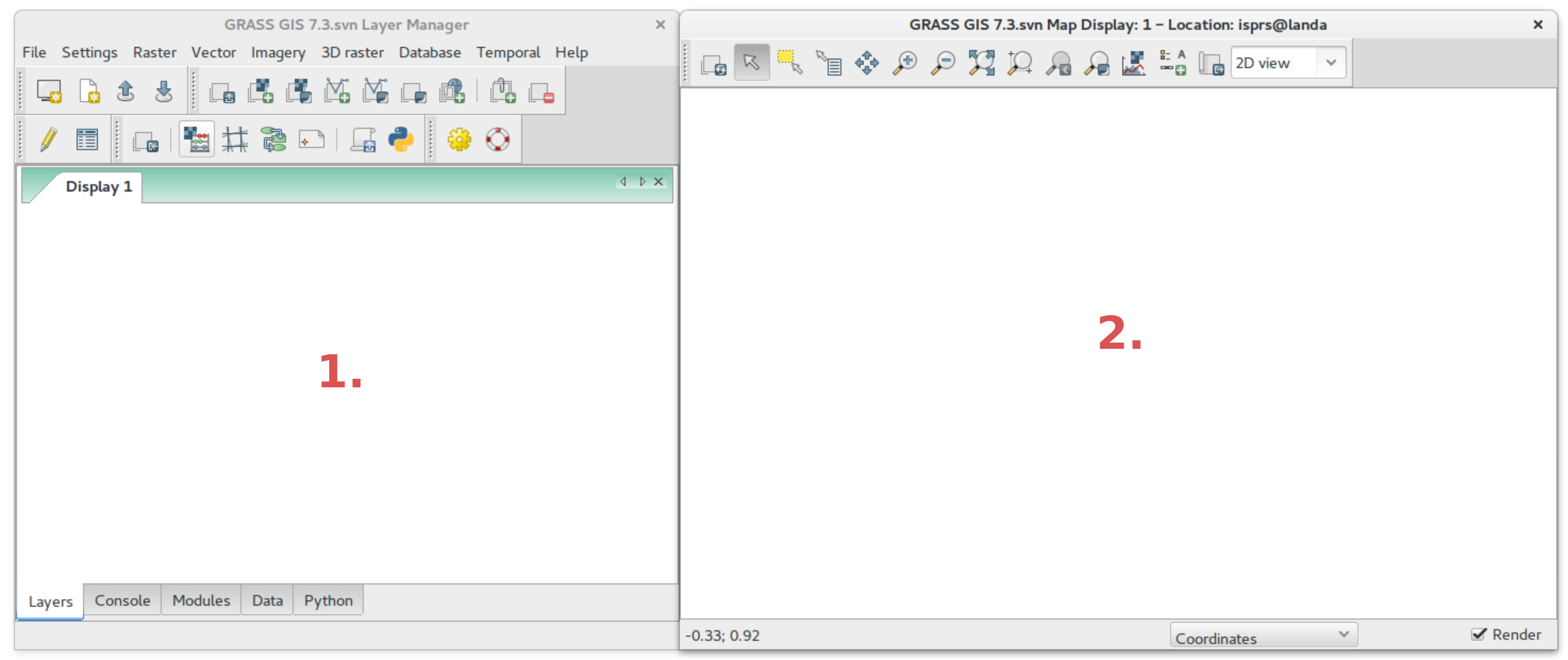
Fig. 23 Layer Manager and Map Display GUI components.

Vector maps can be added similarly to rasters from File ‣ Map display ‣ Add vector, or from the Layer Manager toolbar .

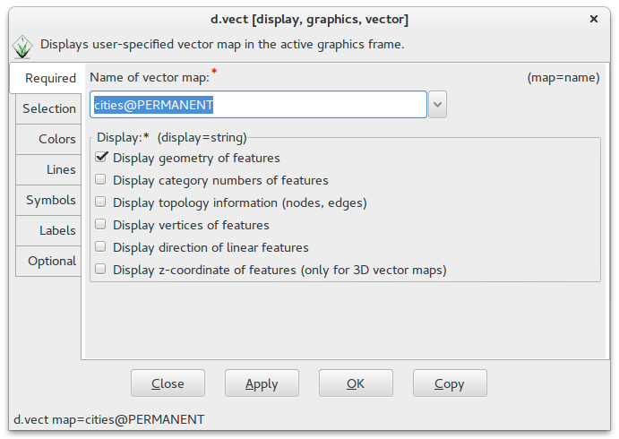
Fig. 24 Dialog (d.vect) for displaying vector data in the Map Display.

Raster maps can be added to layer tree from menu File ‣ Map display ‣ Add raster, or from the Layer Manager toolbar .

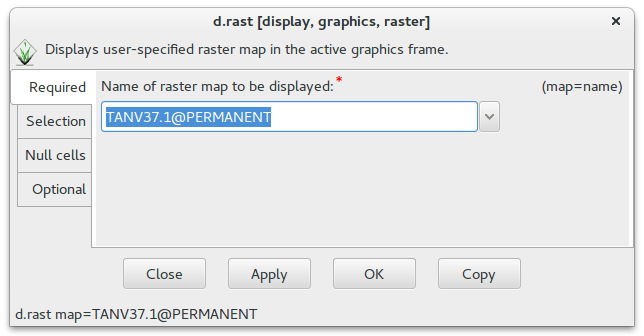
Fig. 25 Dialog (d.rast) for displaying raster data in the Map Display.

RGB orthophotos has been spitted by GRASS into three separate raster maps:

• red channel (.1)
• green channel (.2)
• blue channel (.3)

You can also add multiple raster or vector maps from Layer Manager toolbar by .

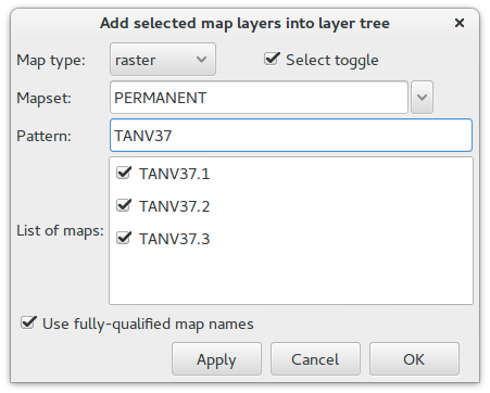
Fig. 26 Add multiple raster maps to layer tree.

RGB composition can be added from Layer Manager toolbar by .

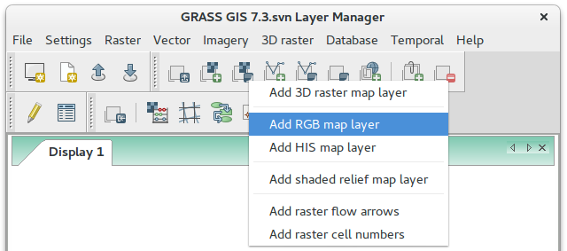
Fig. 27 Add RGB layer.

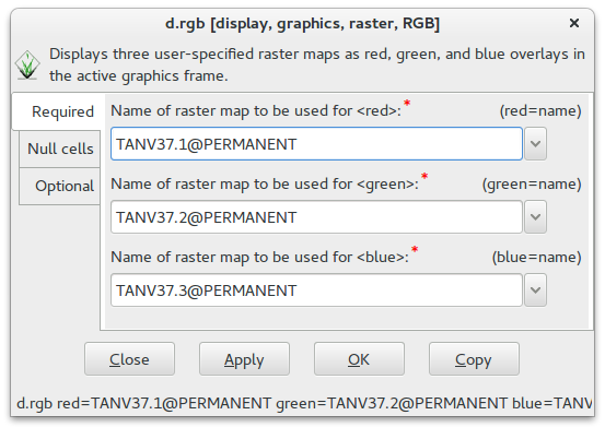
Fig. 28 Compose raster maps to RGB.

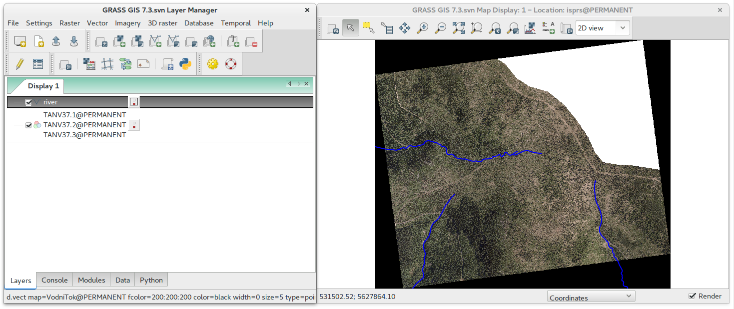
Fig. 29 Example of data visualization.

Accessing GRASS Modules

GRASS is modular system which consists of several hundreds tools (called “modules”). They are accessible from the Layer Manager menu, “Modules” tab, and from command prompt (“Console” tab).

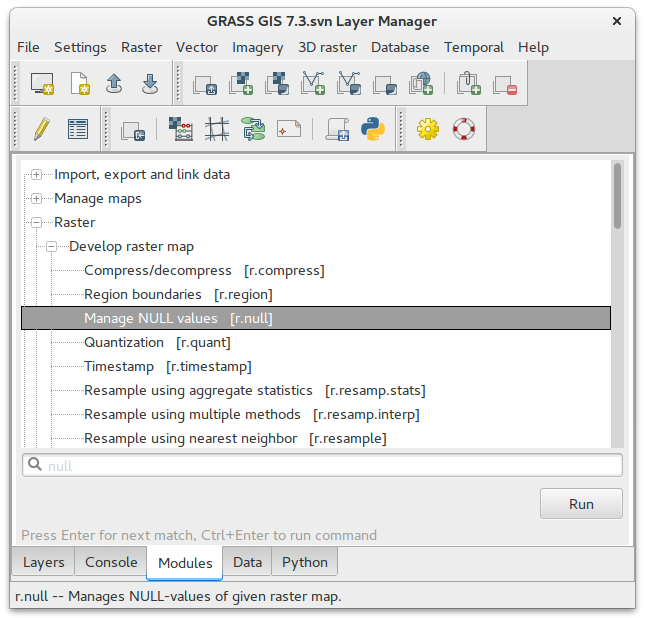
Fig. 30 Searching module in Layer Manager.

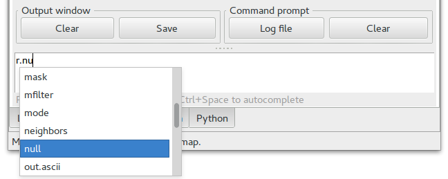
Fig. 31 Launching module from Layer Manager console.

The commands (modules) can be called from GUI dialogs and from command line. Figure bellow shows GUI dialog of r.null module. The equivalent command for console would be:

r.null map=TANV37.1 setnull=0,255

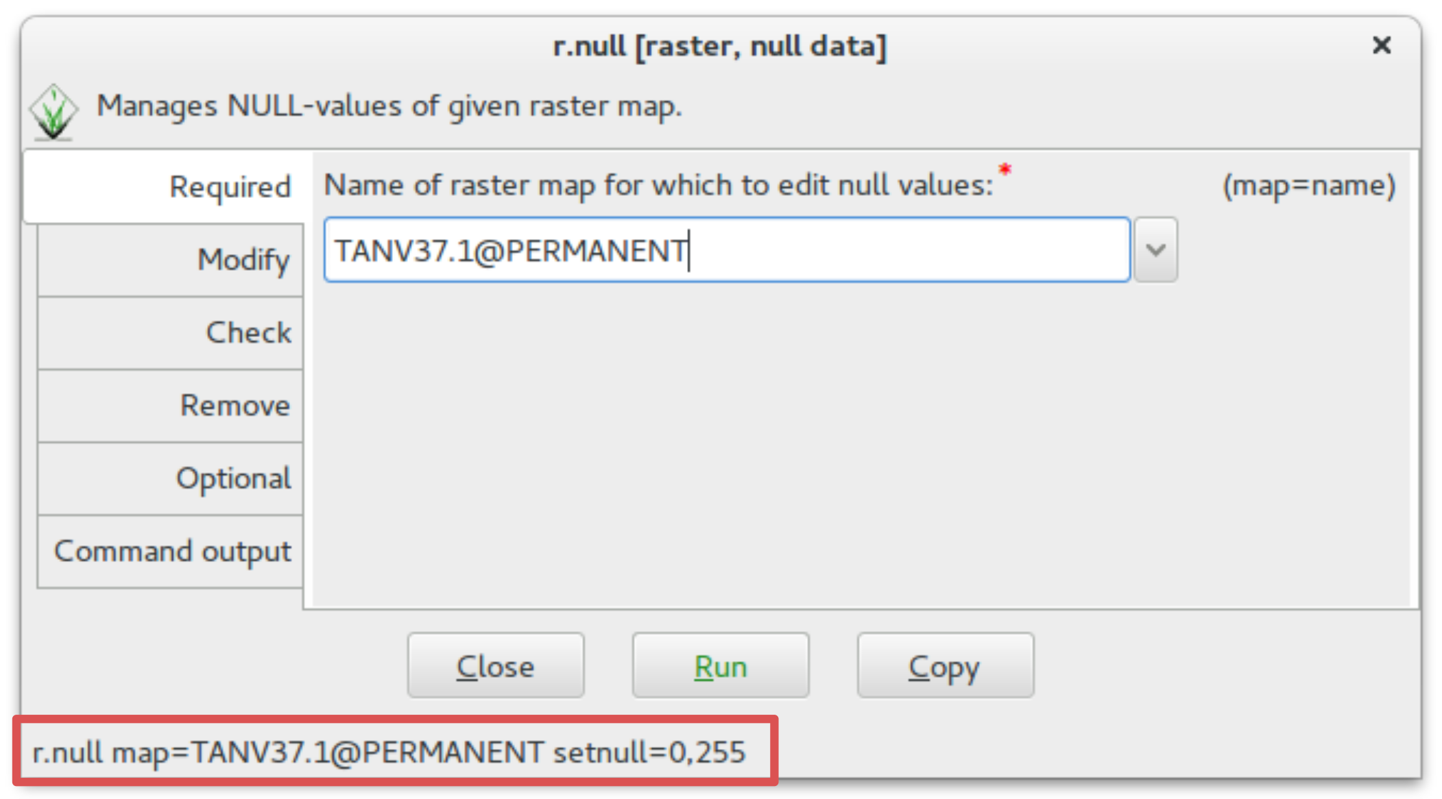
Fig. 32 Dialog of r.null module.

Note

This command replaces in raster maps occurrence of 0 a 255 values by NULL value (no-data). Note that before running this command you need to set up computational region based on selected raster map (g.region).

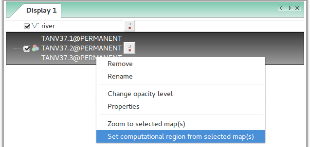
Fig. 33 Set computational region from RGB composition.

Also note that all three raster maps in composition should be modified by r.null. This operation can be automated by Graphical Modeler or by scripting in Python, see Lesson 3 for details.

Performing NULL propagation can introduce holes into image. One of solutions would be to create RGB composition using r.composite and fill holes with combination of r.neighbors (method=mode) and r.mapcalc, example bellow.

r.composite red=TANV37.1 green=TANV37.2 blue=TANV37.3 output=TANV37
r.neighbors input=TANV37 output=TANV37_mode method=mode
r.mapcalc expression="TANV37_final = if ( isnull( TANV37.1 + TANV37.2 + TANV37.3 ), TANV37_mode, TANV37 )"
r.colors map=TANV37_final raster=TANV37

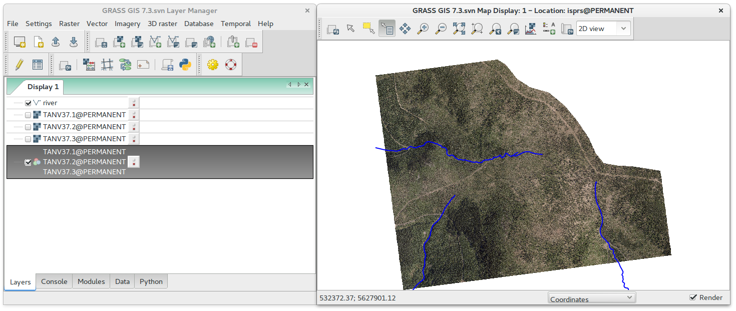
Fig. 34 Result of replacing 0 a 255 values by no-data value.

Working with vector attributes

Tool for browsing and modifying attribute data of vector features is accessible from the layer contextual menu Attribute data or from the Layer Manager toolbar .

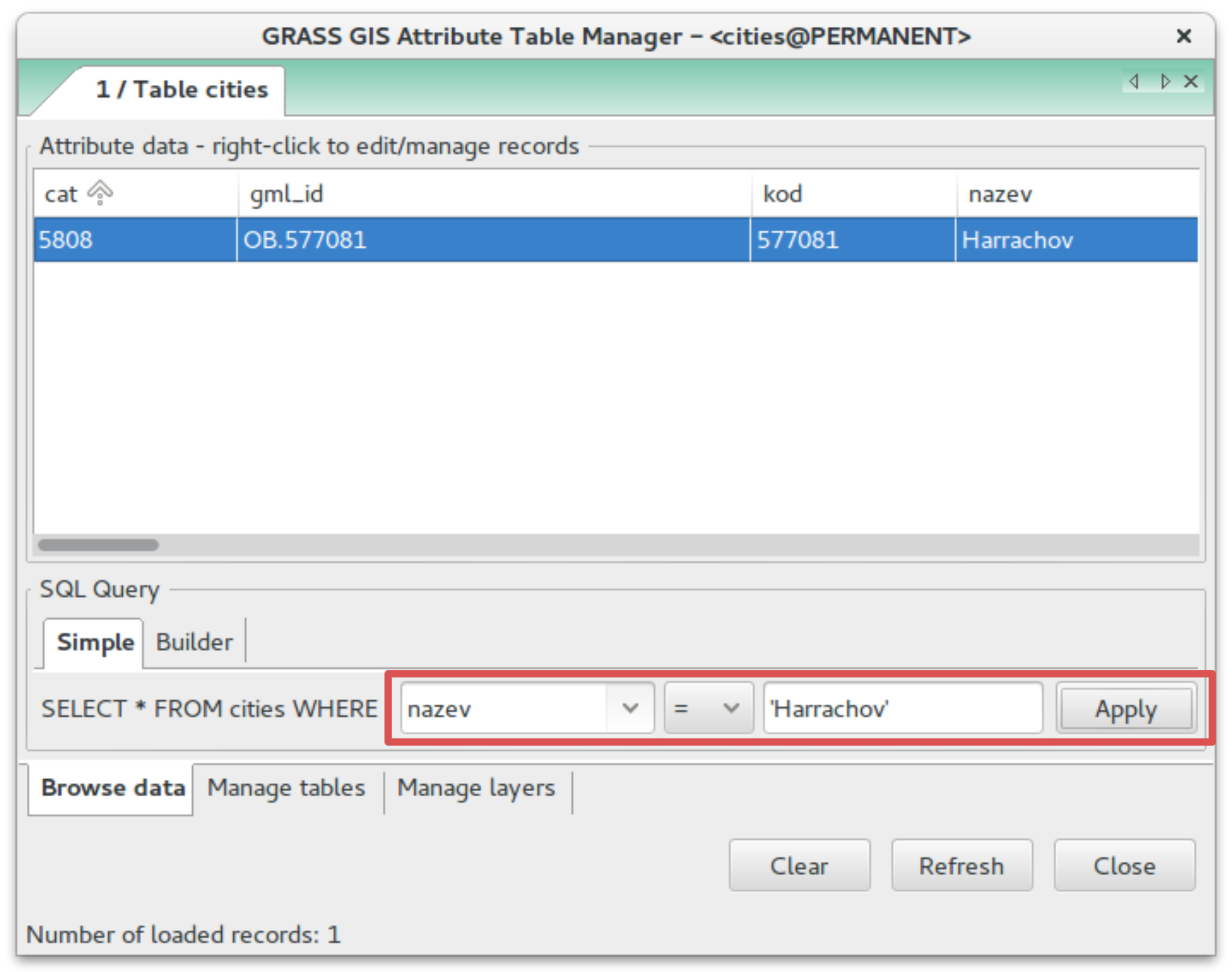
Fig. 35 Example of selecting city Harrachov.

Note

One of GRASS mottos is “Everything what is possible to perform using GUI is possible to reproduce in command line”. For example the operation presented above can be reproduced by v.extract command.

v.extract input=cities where="nazev = 'Harrachov'" output=harrachov

QGIS Plugin

GRASS plugin enables QGIS to access raster and vector data in GRASS format, to display them, browse, and modify including topological editing. The plugin also allows launching GRASS tools (modules) directly from QGIS user interface.

Note

We highly recommend QGIS version 2.14 or higher (this version of QGIS is the first which comes with GRASS 7 included).

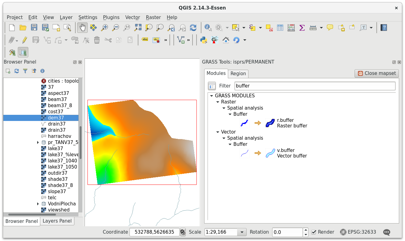
Fig. 36 QGIS GRASS plugin in action.