Unit 17 - Spatio-temporal intro

GRASS GIS offers specialized tools for spatio-temporal data processing, see GRASS documentation for details.

GRASS introduces three special data types that are designed to handle time-series data:

• Space-time raster datasets (strds) for managing raster map time series.
• Space-time 3D raster datasets (str3ds) for managing 3D raster map time series.
• Space-time vector datasets (stvds) for managing vector map time series.

Spatio-temporal flooding simulation

Module r.lake itself allows to generating only one level (represented by one raster map) within one run. This limitation is surpassed by addon r.lake.series.

Note

Addons modules are not internal part of GRASS installation. Addons can be easily installed by g.extension (Settings ‣ Addons extensions ‣ Install extension from addons).

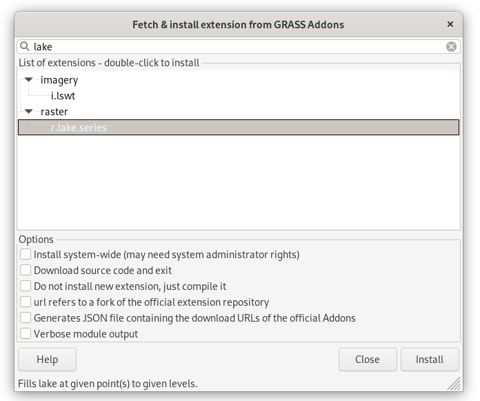
Fig. 100 Install r.lake.series GRASS Addon.

r.lake.series module outputs multiple raster maps registered in space-time raster dataset.

r.lake.series elevation=dem out=lakes start_water_level=134 end_water_level=145 \
 water_level_step=0.1 coordinates=686668,5650664 \
 time_step=10 nproc=3

In the example above we created space-time series between water levels 134 and 145 with step 0.1 m. Time step is 10 min. To increase computation speed we used three CPU cores. The result is stored in raster space-time dataset named lakes.

Basic information about output space-time dataset can be obtained by t.info command.

t.info input=lakes

...
+-------------------- Relative time -----------------------------------------+
| Start time:................. 1
| End time:................... 1101
| Relative time unit:......... minutes
| Granularity:................ 10
| Temporal type of maps:...... point
...

Time topology information can be obtained by t.topology.

t.topology input=lakes

...
+-------------------- Temporal topology -------------------------------------+
...
| Number of points: .......... 111
| Number of gaps: ............ 110
| Granularity: ............... 10
...

Space-time Data Querying

By t.rast.list can be printed raster maps within given time period. In the example below are printed raster maps within the first hour of simulated flooding.

t.rast.list input=lakes order=start_time where="start_time < 60"

Univariate statistic can be calculated by t.rast.univar, in example below statistics is computed only for the first hour of flooding.

t.rast.univar input=lakes where="start_time < 60"

id|start|end|mean|min|max|mean_of_abs|stddev|variance|coeff_var|sum|null_cells|cells
lakes_134.0@flooding|1|None|0.211415510911208|0.007537841796875|0.738616943359375|...
lakes_134.1@flooding|11|None|0.397385983853727|0.000823974609375|1.14051818847656|...
lakes_134.2@flooding|21|None|0.445528310686884|0.0003814697265625|1.24050903320312|...
lakes_134.3@flooding|31|None|0.502563093844781|0.0012054443359375|1.34051513671875|...
lakes_134.4@flooding|41|None|0.564594079032162|0.0021820068359375|1.44050598144531|...
lakes_134.5@flooding|51|None|0.582153865733045|0.0008697509765625|1.54051208496094|...

Data aggregation can be performed by t.rast.aggregate. In the example below data is aggregated by 1 hour.

t.rast.aggregate input=lakes output=lakes_h basename=ag granularity=60 nproc=3

The command generates a new space time dataset which can be used for subsequent analysis like univariate statistics:

t.rast.univar input=lakes_h

id|start|end|mean|min|max|mean_of_abs|stddev|variance|coeff_var|sum|null_cells|cells
ag_00001@flooding|1|61|0.431898174745821|0.0008697509765625|1.34051208496094|...
...
ag_00019@flooding|1081|1141|5.69696318836018|4.57763671875e-05|11.9405110677083|...

Space-time Data Extracting

Raster space-time data can be extract into new datasets using t.rast.extract. In the example below three new datasets are created for the first, second and third six hours of flooding.

t.rast.extract input=lakes where="start_time > 0 and start_time < 361" output=lakes_1
t.rast.extract input=lakes where="start_time > 360 and start_time < 720" output=lakes_2
t.rast.extract input=lakes where="start_time > 720" output=lakes_3

Aggregation into single raster output can be performed by t.rast.series:

t.rast.series input=lakes_1 output=lakes_1_avg method=average

Let’s print univariate statistics for generated raster output by r.univar:

r.univar map=lakes_1_avg

minimum: 0.00152588
maximum: 2.93515
range: 2.93362
mean: 1.0993

Space-time Data Visualization

Time series can be visualized by specialized tool g.gui.timeline. Example below.

g.gui.timeline inputs=lakes_1,lakes_2,lakes_3

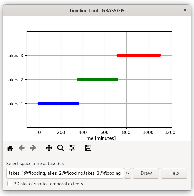
Fig. 101 Timeline tool showing three space-time datasets.

And finally, a simple animation can be created by g.gui.animation (File ‣ Animation tool), see Fig. 102.

g.gui.animation strds=lakes

Fig. 102 Example of flooding animation.