Unit 29 - GRASS GIS and R
R or RStudio can be used in conjunction with GRASS GIS in two different ways:
- run R within a GRASS GIS session
- run GRASS GIS within a R session
In any case a R package called rgrass7 must be installed. Start R within running GRASS session:
R
From R session install (including dependencies) and load the rgrass7 package
install.packages("rgrass7", dependencies=TRUE)

library(rgrass7)
Note
If GRASS GIS is started from R (or RStudio) session a initGRASS()
function must be called in order to define GRASS GIS environment
settings. First get the full path to GRASS GIS installation and run
the initGRASS() function with specified parameters pointing to
GRASS location and mapset to be used.
# Get GRASS library path
grasslib <- try(system('grass --config', intern=TRUE))[4]

initGRASS(gisBase=grasslib, gisDbase='/home/user/grassdata/',
          location='oslo-region', mapset='PERMANENT', override=TRUE)
At this point GRASS GIS modules are available inside R by
execGRASS() function. In example below are listed available vector
maps from the current location and mapset using
g.list. Vector map of administrative regions
(Fylke) is converted to raster format by v.to.rast.
execGRASS("g.list", parameters = list(type = "vector"))
execGRASS("g.region", parameters = list(vector="Fylke", align="modis_avg@modis"))
execGRASS("v.to.rast", parameters = list(input = "Fylke",
          output="fylke", use="cat", label_column="navn"))
GRASS raster map can be read as an R object by readRAST()
function. The cat parameter indicates which raster values to be
returned as factors.
ncdata <- readRAST(c("fylke", "modis_avg@modis"), cat=c(TRUE, FALSE))
summary(ncdata)
Object of class SpatialGridDataFrame
Coordinates:
      min     max
[1,] -572752 1039248
[2,] 5539179 7836179
Is projected: TRUE
proj4string :
[+proj=utm +no_defs +zone=33 +a=6378137 +rf=298.257222101
 +towgs84=0,0,0,0,0,0,0 +to_meter=1]
Grid attributes:
   cellcentre.offset cellsize cells.dim
1           -572252     1000      1612
2           5539679     1000      2297
Data attributes:
                     fylke           modis_avg
  (1:Nordland)          :  80964   Min.   :-11.1
  (1:Trøndelag)         :  58662   1st Qu.: -1.7
  (2:Troms,Romsa)       :  40760   Median :  4.2
  (2:Finnmark,Finnmárku):  31257   Mean   :  3.4
  (1:Hedmark)           :  27403   3rd Qu.:  8.7
  (Other)               : 187401   Max.   : 16.1
  NA's                  :3276317   NA's   :2450449
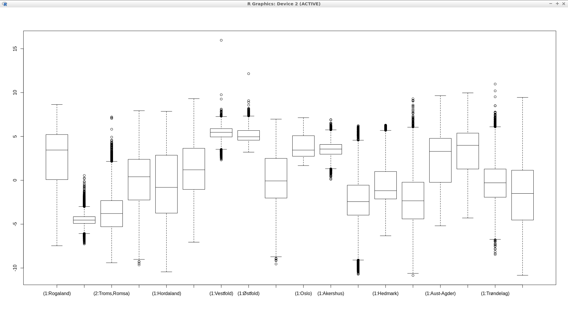
In example below a boxplot of Norwegian regions with the 2017 annual mean values of MODIS LST is ploted, see Fig. 135.
boxplot(ncdata$modis_avg ~ ncdata$fylke, medlwd = 1)
A common use case in ecological analysis is to extract raster values at vector points, e.g. to put sampling locations into spatial context. Using GRASS GIS you can read raster values at point locations directly into R for further analysis (e.g. regression) or plotting.
# First, let`s fetch some sample example data. Lets get data on two species
# from GBIF (gbif.org):
execGRASS('g.region', vector='oslo', flags = 'p')

execGRASS('v.in.pygbif', output='gbif_species', taxa='Rubus chamaemorus,Lotus corniculatus',
          rank='species')

# Extract average temperature from MODIS
execGRASS('v.what.rast', map='gbif_species', raster='modis_avg@modis', column='modis_c_avg')

# query raster maps at vector points, transfer result into R
goutput <- execGRASS('v.db.select', map='gbif_species', columns='g_species,modis_c_avg',
                     where='modis_c_avg IS NOT NULL', separator='comma', intern=TRUE)

# Parse results
con <- textConnection(goutput)
go1 <- read.csv(con, header=TRUE)
str(go1)

# From here you can visualize / analysze in R

# Query time series at vector points, transfer result into R
modis_c_studenterhytta <- execGRASS("t.rast.what", flags=c("n", "i", "overwrite"),
                                    strds="modis_c", nprocs=1,
                                    coordinates=c(592409.49, 6655332.75),
                                    separator='comma', intern=TRUE)

# Parse the result
con <- textConnection(modis_c_studenterhytta)
go2 <- read.csv(con, header=TRUE)
str(go2)
More information and examples can be found at
- the GRASS/rgrass7 wiki page and
- the rgrass7 package documentation
R vs. Python
Python and R are both popular languages for data science. And the question which language to use (and for what purposes) has often been discussed, e.g. at Data-Driven Science or Dataquest . There, Python and R are often considered as complementing each other with R being stronger on data visualisation and statistics while Python is considered more general purpose programming language with advantages in performance. For more computational demanding processes, Python can have significant advantages, esp. if looping is involved as the following example illustrates:
# Create a simple loop-script in R
echo 'library("iterpc")
it <- iterpc(10000, 2, replace=TRUE)

for (i in getall(it)) {
    iN <- i[1]
}' > loop.r

# Create a simple loop-script in Python
echo 'import itertools

it = itertools.combinations(range(0,10000),2)
for i in it:
    iN = i[0]' > loop.py
Run the R script while tracing memory usage
./memusg Rscript loop.r
memusg: peak=436312
Run the Python script while tracing memory usage
./memusg python loop.py
memusg: peak=5528
Run the Python script and measure execution time
time python loop.py
real    0m4.516s
user    0m4.506s
sys     0m0.004s
Run the R script and measure execution time
time Rscript loop.r
real    0m36.733s
user    0m36.084s
sys     0m0.273s
As you can see, in the case above, R uses ~80 times more memory and takes ~9 times longer to complete the loop-test above.
For people coming from ‘’R’’ the ‘’Python’’ library ‘’pandas’’ is worth exploring. It provides data organisation and methods very similar data frames in ‘’R’‘.
Getting started with ‘’Python’’ and ‘’pandas’’ gets easy with the Pandas Cheat Sheet or a more general Python cheat sheet from DataScience.
A nice comparison between R and functions/data management offered by pandas library can be found here.
For getting a basic, hands-on introduction to Python Codeacademy can be recommended as a free learning platform.