Unit 27 - Regression analysis
GRASS GIS comes with different modules performing regression analysis. These modules work with single raster map or with time series data too. There are two core GRASS modules related to regression: r.regression.line and r.regression.multi. There are also other interesting modules distributed as addons which will be demostrated in this unit.
r.regression.line
r.regression.line calculates a linear regression from two raster maps, according to the formula y = a + b*x. It also returns some regression coefficients like offset/intercept (a), gain/slope (b), correlation coefficient (R), number of elements (N), means (medX, medY), standard deviations (sdX, sdY), and the F test for testing the significance of the regression model as a whole (F); these parameters could be saved in a text file.
r.regression.line mapx=dtm mapy=modis_avg
y = a + b*x
a (Offset): 6.534392
b (Gain): -0.009867
R (sumXY - sumX*sumY/N): -0.862133
N (Number of elements): 718021
F (F-test significance): 2078811.252064
meanX (Mean of map1): 269.004369
sdX (Standard deviation of map1): 129.487450
meanY (Mean of map2): 3.880192
sdY (Standard deviation of map2): 1.481930
It is possible to apply the model variable with the predictor
r.mapcalc expression="temp_linear = 6.534392 + -0.0096867 * dtm"
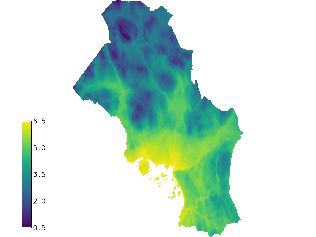
Fig. 124 Model variable with predictor example.
Tip
In Linux Bash eval command allows to store an output of GRASS GIS modules called with -g flag as environmental variables which can be reused afterwards by other GRASS modules, see example below.
eval `r.regression.line -g mapx=dtm mapy=modis_avg`
r.mapcalc expression="temp_linear = $a + $b * dtm"
r.regression.multi
The r.regression.multi calculates a multiple linear regression from raster maps according to the formula Y = b0 + sum(bi*Xi) + E. Two output maps are returned, one for residuals and one for estimates plus all the regression coefficients.
Create a map with maximum NDVI value from spatio-temporal dataset created in Unit 23 - Spatio-temporal NDVI by t.rast.series.
g.region vector=oslo align=L2A_T32VNM_20170506T105031_B04_10m
t.rast.series input=ndvi_cloud method=maximum output=ndvi_max
And now use the maximum NDVI map as one of the input coefficients.
r.regression.multi mapx=dtm,ndvi_max mapy=modis_avg residuals=resi estimates=esti -g
n=4353047
Rsq=0.749059
Rsqadj=0.749059
RMSE=0.746155
MAE=0.593534
F=6496914.853654
b0=6.792572
AIC=-2549329.836898
AICc=-2549329.836898
BIC=-2549289.977738

predictor1=dtm
b1=-0.009514
Rsq1=0.583921
F1=10129206.204638
AIC1=2683241.367502
AICc1=2683241.367502
BIC1=2683252.653888

predictor2=ndvi_max
b2=-0.497951
Rsq2=0.006463
F2=112121.300410
AIC2=-2438630.088387
AICc2=-2438630.088387
BIC2=-2438618.802001
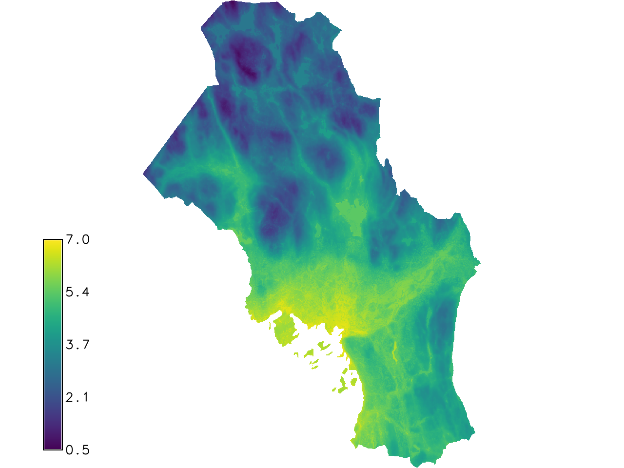
Fig. 125 The estimates output by r.regression.multi.
Tip
It is possible to calculate differences between original LST data and the output of the models with r.mapcalc.
r.gwr
There two GRASS Addons modules related to regression analysis: r.gwr and r.regression.series.
r.gwr calculates geographically weighted regression from raster maps, it resolves a formula Y = b0 + sum(bi*Xi) + E. The formula is applied in a moving window. Cells closer to the center of the moving window get a higher weight. r.gwr is more an analytical tool to test if the predictors are suitable for a global model applied by r.regression.multi.
r.gwr mapx=dem,ndvi_max mapy=modis_avg residuals=resi_gwr estimates=esti_gwr -g
n=4321368
Rsq=0.997701
Rsqadj=0.997701
F=9.37847e+08
bmean0=-4.35557
bstddev0=2863.45
bmin0=-3.58167e+06
bmax0=495224
AIC=-2.27972e+07
AICc=-2.27972e+07
BIC=-2.27972e+07
predictor1=dtm
bmean1=0.0330626
bstddev1=12.7136
bmin1=-2005.55
bmax1=14986.4
Rsq1=4.38811e-05
F1=82497.2
AIC1=-2.27155e+07
AICc1=-2.27155e+07
BIC1=-2.27155e+07
predictor2=ndvi_max
bmean2=-0.0112723
bstddev2=0.773451
bmin2=-123.338
bmax2=43.0038
Rsq2=1.02995e-05
F2=19363.3
AIC2=-2.27779e+07
AICc2=-2.27779e+07
BIC2=-2.27779e+07
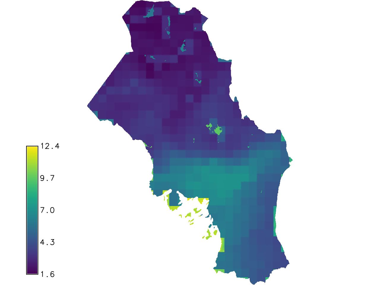
Fig. 126 The estimates output produced by r.gwr.
r.regression.series
r.regression.series calculates linear regression parameters from two space time raster datasets. The module makes each output cell value a function of the values assigned to the corresponding cells in the two input raster map series. Following methods are available:
- offset: Linear regression offset
- slope: Linear regression slope
- corcoef: Correlation Coefficent R
- rsq: Coefficient of determination = R squared
- adjrsq: Adjusted coefficient of determination
- f: F statistic
- t: T statistic
Before to running r.regression.series two it is needed to prepare the two sample space time raster datasets. There is dataset ndvi_cloud created in Unit 23 - Spatio-temporal NDVI which could be used.
t.rast.list ndvi_cloud
name|mapset|start_time|end_time
ndvi_cloud_1|PERMANENT|2017-05-06 10:50:31|2017-05-06 10:50:32
ndvi_cloud_2|PERMANENT|2017-05-23 10:40:31|2017-05-23 10:40:32
ndvi_cloud_3|PERMANENT|2017-05-26 10:50:31|2017-05-26 10:50:32
ndvi_cloud_4|PERMANENT|2017-07-05 10:50:31|2017-07-05 10:50:32
Another dataset which could be used is modis_c created in Unit 22 - Spatio-temporal basic analysis. For our purpose it is more reasonable to calculate the mean value for each eight days. This calculation can be done by Python script below.
1 2 3 4 5 6 7 8 9 10 11 12 13 14 15 16 17 18 19 20 21 22 23 24 25 26 27 28 29 30 31 32 33 34 35 36 37 38 39 40 41 42 43 44 45 46 47 48 49 50 51 52 53 54 55 56 57 58 59 60 61 62 63 64 65 66 67 68 69 70 71 72 73 74 75 76 77 78 79 80 81 82 83 84 85 86 87 88 89 90 91 92 93 94 95 96 97 98 | #!/usr/bin/env python
#%module
#% description: Computes aggregation for maps
#%end
#%option G_OPT_STRDS_INPUT
#%end
#%option G_OPT_STRDS_OUTPUT
#%end
#%option
#% key: basename
#% description: Basename for output raster maps
#% required: yes
#%end
#%option
#% key: method
#% description: Aggregate operation to be performed on the raster maps
#
#% required: yes
#% multiple: no
#% answer: average
#% type: string
#%end
#%option
#% key: nprocs
#% description: Number of processes
#% answer: 1
#% type: integer
#%end
import os
import sys
import atexit
import grass.script as gcore
from grass.pygrass.modules import Module, MultiModule, ParallelModuleQueue
date_format = "%Y-%m-%d %H:%M:%S"
def calculate(inp, dat, out, out_rast, met):
modules = []
modules.append(
Module('t.rast.series',
input=inp.get_name(),
method=met,
output=out_rast,
where="start_time >= '{st}' and end_time <= '{se}'".format(
st=dat[0].strftime(date_format),
se=dat[1].strftime(date_format)),
run_ = False
)
)
queue.put(MultiModule(modules, sync=False))
def main():
import grass.temporal as tgis
tgis.init()
dbif = tgis.SQLDatabaseInterfaceConnection()
dbif.connect()
inp = tgis.open_old_stds(options['input'], 'raster')
temp_type, sem_type, title, descr = inp.get_initial_values()
out = tgis.open_new_stds(options['output'], 'strds', temp_type,
title, descr, sem_type, dbif=dbif,
overwrite=gcore.overwrite())
dates = []
for mapp in inp.get_registered_maps_as_objects():
if mapp.get_absolute_time() not in dates:
dates.append(mapp.get_absolute_time())
dates.sort()
idx = 1
out_maps = []
for dat in dates:
outraster = "{ba}_{su}".format(ba=options['basename'], su=idx)
out_maps.append(outraster)
calculate(inp, dat, out, outraster, options['method'])
idx += 1
queue.wait()
times = inp.get_absolute_time()
tgis.register_maps_in_space_time_dataset('raster', out.get_name(),
','.join(out_maps),
start=times[0].strftime(date_format),
end=times[1].strftime(date_format),
dbif=dbif)
if __name__ == "__main__":
options, flags = gcore.parser()
# queue for parallel jobs
queue = ParallelModuleQueue(int(options['nprocs']))
sys.exit(main())
|
Sample script to download: lst_average.py
Example of usage:
lst_average.py input=modis_c output=modis_c_days basename=modis_days
At this point select four raster maps close to the NDVI maps:
t.rast.list modis_c_days where="start_time >= '2017-05-01 00:00:00' and end_time <= '2017-07-20 00:00:00'"
name|mapset|start_time|end_time
modis_days_16|PERMANENT|2017-05-01 00:00:00|2017-05-09 00:00:00
modis_days_17|PERMANENT|2017-05-09 00:00:00|2017-05-17 00:00:00
modis_days_18|PERMANENT|2017-05-17 00:00:00|2017-05-25 00:00:00
modis_days_19|PERMANENT|2017-05-25 00:00:00|2017-06-02 00:00:00
modis_days_20|PERMANENT|2017-06-02 00:00:00|2017-06-10 00:00:00
modis_days_21|PERMANENT|2017-06-10 00:00:00|2017-06-18 00:00:00
modis_days_22|PERMANENT|2017-06-18 00:00:00|2017-06-26 00:00:00
modis_days_23|PERMANENT|2017-06-26 00:00:00|2017-07-04 00:00:00
modis_days_24|PERMANENT|2017-07-04 00:00:00|2017-07-12 00:00:00
modis_days_25|PERMANENT|2017-07-12 00:00:00|2017-07-20 00:00:00
Finally it is possible to run r.regression.series using several methods to get various outputs.
r.regression.series xseries=ndvi_cloud_1,ndvi_cloud_2,ndvi_cloud_3,ndvi_cloud_4 \
yseries=modis_days_16,modis_days_18,modis_days_19,modis_days_24 \
method=offset,slope,rsq output=temp_offset,temp_slope,temp_rsq
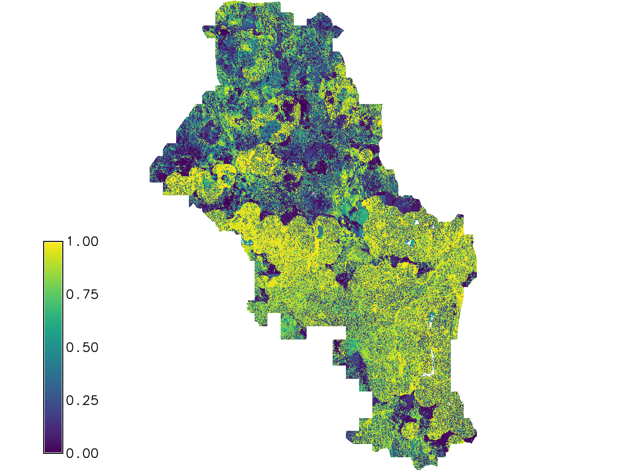
Fig. 127 The output RSQ value.