Unit 19 - Sentinel preprocessing
In this unit Sentinel-2 L1C (see Sentinel Product Types description) data will be preprocessed to be used in GRASS GIS.
In the first step few Sentinal scenes will be downloaded similarly as shown in Unit 18 - Sentinel downloader. In this case producttype=S2MSI2Ap will be replaced by producttype=S2MSI1C.
i.sentinel.download -l map=oslo producttype=S2MSI1C settings=sentinel.txt \
start=2018-04-01 end=2018-10-01 area_relation=Contains clouds=10
ef0b12ac-9c79-46ec-8223-9655791943ea 2018-05-18T10:40:21Z  0% S2MSI1C
...
97a5820c-c1c8-4300-a076-174c9e7694fa 2018-05-23T10:40:19Z  0% S2MSI1C
...
d6ab2378-84e8-4e73-8be9-0e9833587a65 2018-06-02T10:40:19Z  9% S2MSI1C
Since we already have the Sentinel scene for 23rd May (Unit 18 - Sentinel downloader) and 5th July 2017 (Unit 05 - Simple computation) the same dates of 2018 can be downloaded. A command to download specified scenes by UUID below.
i.sentinel.download settings=sentinel.txt output=geodata/sentinel/2018 \
uuid=97a5820c-c1c8-4300-a076-174c9e7694fa
In the next step downloaded data are imported into GRASS GIS using another command provided by i.sentinel addons, i.sentinel.preproc. This module requires some inputs used to perform the atmospheric correction of Sentinel-2 images.
As elevetion model DMT imported in Unit 17 can be used. What we need to obtain yet is a visibility map or an Aerosol Optical Depth (AOD) value, the second one is possible to get from http://aeronet.gsfc.nasa.gov.
First you have to select a station close to your Sentinel-2 scene area. In our case Birkenes, click on download, see Fig. 110.
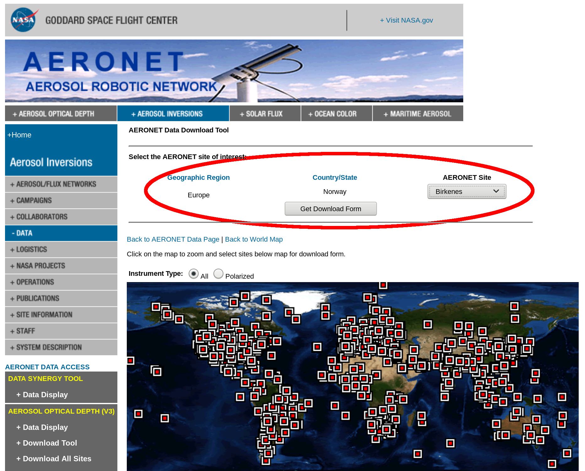
Fig. 110 Download Aeronet station data.
Now tick the box near the bottom labelled as ‘Combined file (all products without phase functions)’.
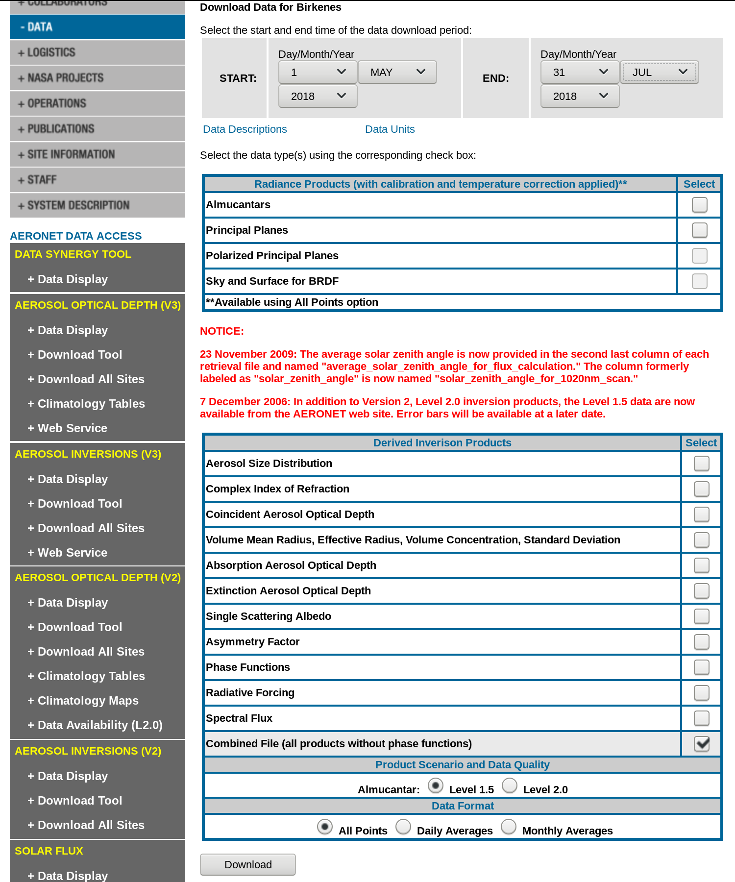
Fig. 111 Combined file requested.
Last step is to accept the license (Public domain data).
Once we have downloaded Sentinel and AOD data we need to decompress
them (it is possible to find already the AOD file in ~/geodata/sentinel/2018/).
cd ~/geodata/sentinel/2018/
unzip S2B_MSIL1C_20180523T104019_N0206_R008_T32VNM_20180523T142657.zip
Now we are ready to import the data with i.sentinel.preproc.
i.sentinel.preproc -a -t \
input_dir=~/geodata/sentinel/S2B_MSIL1C_20180523T104019_N0206_R008_T32VNM_20180523T142657.SAFE \
elevation=DTM_patch atmospheric_model=Automatic aerosol_model="Continental model" \
aeronet_file=~/geodata/sentinel/2018/180501_180531_Birkenes.dubovik suffix=cor \
text_file=~/geodata/sentinel/S2B_MSIL1C_20180523T104019_N0206_R008_T32VNM_20180523T142657.SAFE/mask.txt
Note
In our case DTM from Unit 17 or EU-DEM from Unit 15 - DMT reprojection can be used. In both cases the data needs to be reprojected into sentinel mapset, see How-to reproject data section for details.
The -a flag is needed since we use AOD file, -t is used to write a text file (text_file) ready to be used as input for the next step, creating cloud mask by i.sentinel.mask.
Set the region based on DTM_patched and resolution 10 meters (in the case of EU-DEM set 25 meters).
g.region raster=DTM_patch res=10 -ap
i.sentinel.mask creates clouds and cloud shadows masks for Sentinel-2 images, the algorithm has been developed starting from rules found in literature (Parmes et. al 2017) and conveniently refined.
i.sentinel.mask -r cloud_mask=T32VNM_20180523T104019_cloud shadow_mask=T32VNM_20180523T104019_shadow \
cloud_threshold=25000 shadow_threshold=5000 \
input_file=~/geodata/sentinel/S2B_MSIL1C_20180523T104019_N0206_R008_T32VNM_20180523T142657.SAFE/mask.txt \
mtd_file=~/geodata/sentinel/S2B_MSIL1C_20180523T104019_N0206_R008_T32VNM_20180523T142657.SAFE/MTD_MSIL1C.xml
In the last step topographic correction of reflectance must be performed in order to use Sentinel data for analysis. Required sun position for a given date is computed by r.sunmask.
r.sunmask -gs DTM_patch year=2018 month=5 day=23 hour=10 minute=40 timezone=0
Using map center coordinates: 250000.000000 6675000.000000
...
sunazimuth=167.292191
sunangleabovehorizon=50.010803
sunrise=02:31:19
sunset=19:58:34
The r.sunmask output is returning the sun angle above the horizont (h), instead we need the zenith (z). So we need to do a simple substraction
z = 90 - h
In our example the zenith value is 39.99.
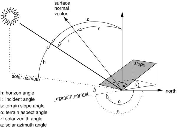
Fig. 112 Figure showing terrain and solar angles. Derived from Neteler & Mitasova, 2008.
Now we have to run i.topo.corr to calculate an illumination model from the elevation map, and finally correct the bands. Pay attention that i.topo.corr requires DCELL (double) raster type so before running i.topo.corr raster type conversion is required. To convert all the maps a sample Python code below can be used.
#!/usr/bin/env python

from grass.pygrass.gis import Mapset
from grass.pygrass.modules import Module

mapset = Mapset()
mapset.current()

# make a for loop for each Sentinel band
for rast in mapset.glist("raster", pattern="T32VNM_20180523T104019_B*_cor"):
    # set compupational region region
    Module("g.region", raster=rast)
    # convert the data
    Module("r.mapcalc", expression="{r}_d=double({r})".format(r=rast))
i.topo.corr -i basemap=DTM_patch zenith=39.99 azimuth=167.292191 output=dtm_illu
i.topo.corr basemap=dtm_illu input=T32VNM_20180523T104019_B08_cor_d,\
T32VNM_20180523T104019_B02_cor_d,T32VNM_20180523T104019_B03_cor_d,T32VNM_20180523T104019_B04_cor_d \
output=tcor zenith=39.99 method=c-factor
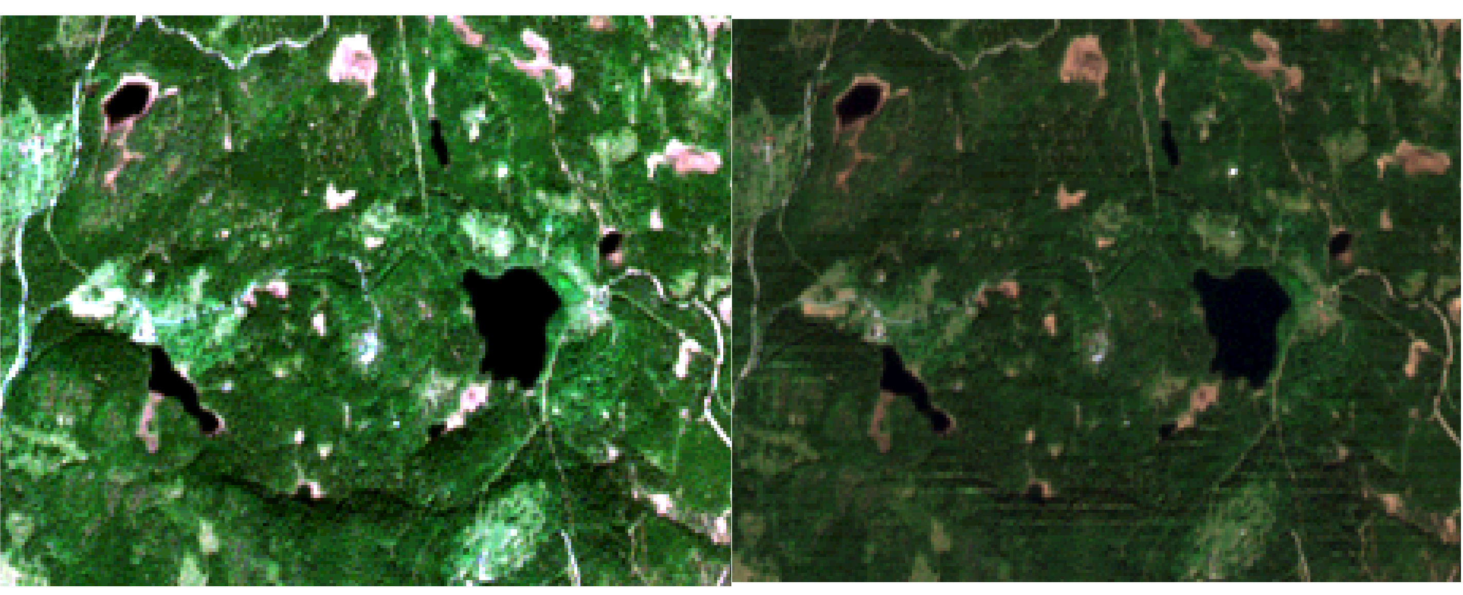
Fig. 113 In the left the original RGB data enhanced by i.color.enhance, in the right the RGB of topographically corrected bands.
Tip
To visualize RGB images read the note at Unit 03. To create RGB raster maps, r.composite can be used.