Unit 04 - Modules, Region
Accessing GRASS modules
GRASS is a modular system which consists of several hundreds tools (called “modules”). Modules are accessible from the Layer Manager menu, Modules tab, or from command prompt (Console tab).
At first import vector cloud mask data layer
MSK_CLOUDS_B00.gml located in sentinel/sample
directory similarly as done in Vector data
(Unit 03 - Data Management).
Warning
MSK_CLOUDS_B00.gml file does not include
information about SRS. It is neccesary to enable Override
projection check before importing data (see Unit 03 for details).
Then find a tool for clipping cloud mask vector map by Oslo region.

Fig. 32 Searching module in Layer Manager by ‘clip’ keyword. The module which we are looking for is v.clip. Module dialog is open by Run button.
Note
Module v.clip has been introduce to GRASS in version 7.4.0. In older versions more generic v.overlay module can be used.
The commands (modules) can be called using GUI dialogs, from command line (Console or “real” terminal), or by using Python API (see Unit 10 - Python intro). Figure bellow shows GUI dialog of v.clip module.

Fig. 33 GUI dialog for launching v.clip module.
Tip
CLI syntax of modules is shown in GUI dialog statusbar, see Fig. 33. Command can be copied to clipboard by Copy button for later usage.
The corresponding command for console would be:
v.clip input=MaskFeature clip=oslo output=oslo_clouds
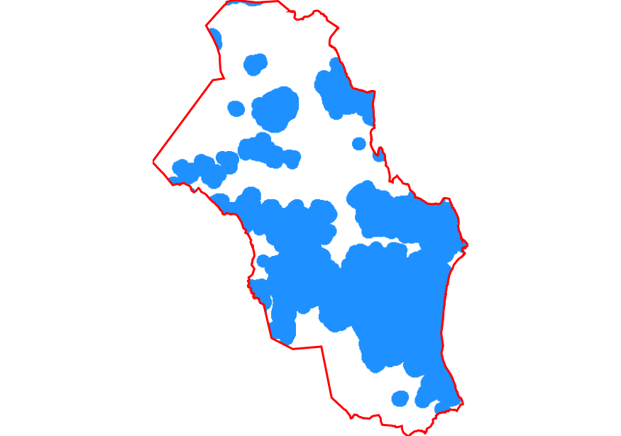
Fig. 34 Clipped clouds mask by Oslo region.
As you can see from example above GRASS commands start by a prefix. This prefix groups modules into several sections, see table below.
| prefix | section | description |
|---|---|---|
db. |
database | attribute data management |
d. |
display | display commands |
g. |
general | generic commands |
i. |
imagery | imagery data processing |
ps. |
postscript | map outputs |
r. |
raster | 2D raster data processing |
r3. |
raster3D | 3D raster data processing |
t. |
temporal | Temporal data processing |
v. |
vector | 2D/3D vector data processing |
Computational region
Computation region is a key issue in GRASS raster processing. Unlike GIS software like Esri ArcGIS which sets computation region based on input data, GRASS is leaving this operation to the user.
Important
The user must define computation region before any raster computation is performed!
Computational region is defined by extent (north, south, east, west) and by spatial resolution in the both directions (east-west, north-south). Note that GRASS supports only regular grids.
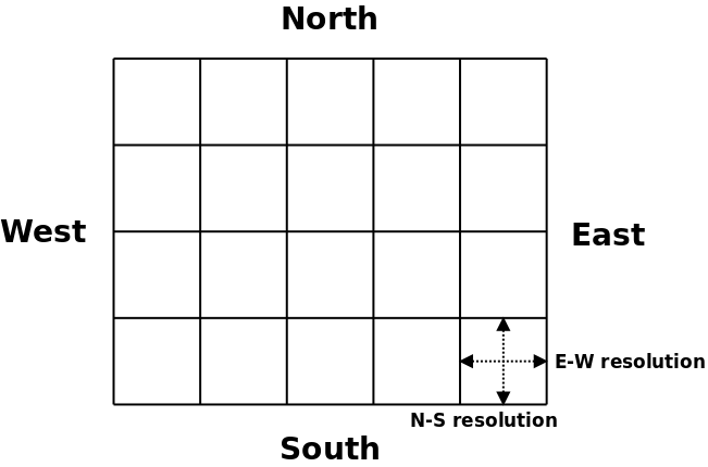
Fig. 35 2D computation region grid.
Note
For 3D raster data (known as “volumes”) there is an extension to 3D computation grid.
Majority of raster processing GRASS modules (r.*) respect
computational region, there are a few exceptions like import modules
(eg. r.import). On the other hand, the most of vector
processing modules (v.*) ignore computation region completely
since there is no computation grid defined by them.
Computational region can be easily set on existing raster or vector map from Layer Manager.
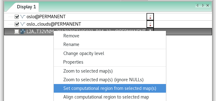
Fig. 36 Set computational region from raster map.
Note that when setting up computational region from vector map, only extent is adjusted. It’s good idea to align the computational grid based on raster map used for computation (Align computational region to selected map).
Tip
Current computation extent can be displayed in map window.
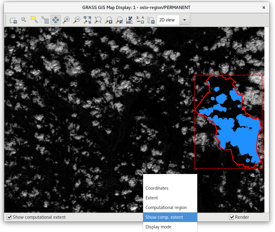
Fig. 37 Show computation region extent in Map Window.
Full flexibility for operating with computation region allows g.region module (). Example below:
g.region vector=oslo align=L2A_T32VNM_20180222T104029_B04_10m
Color table
With knowledge of computational region let’s enhance color table of imported Sentinel band using histogram equalization (which is influenced by computation region as we already know) by using r.colors command.
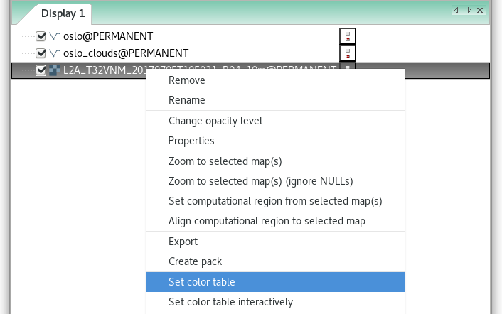
Fig. 38 Set color table from Layer Manager.
Tip
Color table can be easily set also from Layer Manager or managed interactively by .
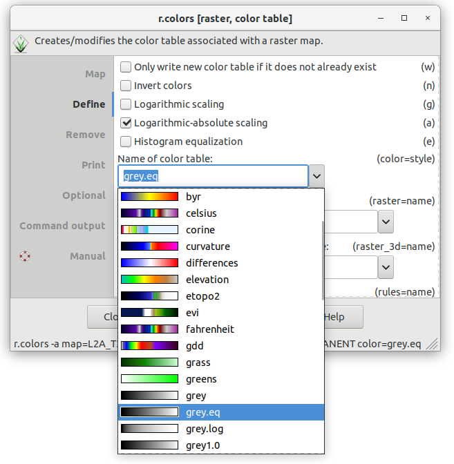
Fig. 39 Set ‘grey.eq’ color table.
r.colors map=L2A_T32VNM_20180222T104029_B04_10m color=grey.eq
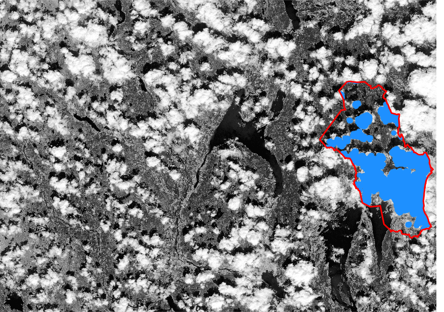
Fig. 40 Sentinel 4th band with enhanced grey color table.